Introduction to time series

In this short article we will take a look at the time series, time series analysis and also time series forecasting in a brief. We will also take a look at some important concepts in time series.

1. Introduction to time series

2. Components of time series

3. Models used to decompose time series

Introduction to Time Series:

What is Time Series?

1. A time series is a series of data points indexed (or listed or graphed) in time order.
   

2. Most commonly, a time series is a sequence taken at successive equally spaced points in time.

3. Thus it is a sequence of discrete-time data. Examples of time series are heights of ocean tides, counts of sunspots, and the daily closing value of the Dow Jones Industrial Average.

4. In the broadest definition, a time series is any data set where the values are measured at different points in time.
   

5. Many time series are uniformly spaced at a specific frequency, for example, hourly weather measurements, daily counts of web site visits, or monthly sales totals.

6. Time series can also be irregularly spaced and sporadic, for example, timestamped data in a computer system’s event log or a history of 911 emergency calls.

7. Pandas time series tools apply equally well to either type of time series.

What is Time Series Analysis?

1. Time series analysis comprises methods for analyzing time series data in order to extract meaningful statistics and other characteristics of the data.

What is Time Series Forecasting?

1. Time series forecasting is the use of a model to predict future values based on previously observed values

2. A stochastic model for a time series will generally reflect the fact that observations close together in time will be more closely related than observations further apart.

3. In addition, time series models will often make use of the natural one-way ordering of time so that values for a given period will be expressed as deriving in some way from past values, rather than from future values

4. Time series analysis can be applied to real-valued, continuous data, discrete numeric data, or discrete symbolic data (i.e. sequences of characters, such as letters and words in the English language).

(Source: Wikipedia)

Example: Actual sell (time series) and Forecast of Sell over the same time period

Note that the following components are important. These terms you will find used in time series analysis or in time series forecasting.

Components of time series:

An observed time series can be decomposed into three components:

1. the trend (long term direction),

2. the seasonal (systematic, calendar related movements) and

3. the irregular (unsystematic, short term fluctuations)

What are seasonal effect? When to apply seasonal adjustments in the time series analysis or in forecasting ?

1. A seasonal effect is a systematic and calendar related effect.

2. Some examples include the sharp escalation in most Retail series which occurs around October or November at the time of Diwali in India, or an increase in water consumption in summer due to warmer weather.

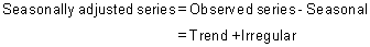
3. Observed data needs to be seasonally adjusted as seasonal effects can conceal both the true underlying movement in the series, as well as certain non-seasonal characteristics which may be of interest to analysts.

4. But when a time series is dominated by the trend or irregular components, it is nearly impossible to identify and remove what little seasonality is present. Hence seasonally adjusting a non-seasonal series is impractical and will often introduce an artificial seasonal element.

Trend:

1. The ‘long term’ movement in a time series without calendar related and irregular effects

2. It can be the result of external influences for example general economic changes, population growth, etc

What is Seasonality?

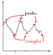
Example peaks and troughs

Seasonality in a time series can be identified by regularly spaced peaks and troughs which have a consistent direction and approximately the same magnitude every year, relative to the trend

The seasonal component consists of effects that are reasonably stable with respect to timing, direction and magnitude. It arises from systematic, calendar related influences such as:

1. Natural Conditions

2. Business and Administrative procedures

3. Social and Cultural behaviour

4. Trading Day Effects

5. Moving Holiday Effects

Note that  the  irregular (or residual) component results from short term fluctuations in the series which are neither systematic nor predictable. In a highly irregular series, these fluctuations can dominate movements, which will mask the trend and seasonality

Models used to decompose time series

Broadly we have two main models used to decompose the observed time series these are as follows:

1. Additive and

2. Multiplicative

3. Pseudo-Additive Decomposition

In the next article I will explain the time series forecasting using Facebook prophet. In prophet we can use one of these two models at the time of forecasting. But main question is when to which one of these models?

Additive:

1. In some time series, the amplitude of both the seasonal and irregular variations do not change as the level of the trend rises or falls. In such cases, an additive model is appropriate. (Example is below figure 4)

2. In the additive model, the observed time series (Ot) is considered to be the sum of three independent components: the seasonal St, the trend Tt and the irregular It.

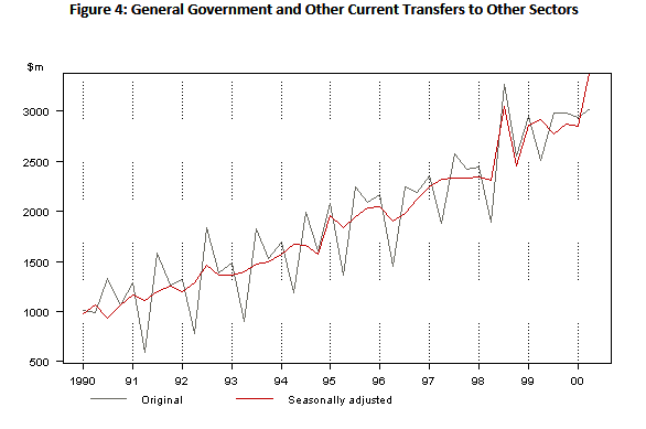
(Source for these figure 4: link)

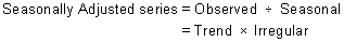
Multiplicative:

1. In many time series, the amplitude of both the seasonal and irregular variations increase as the level of the trend rises. In this situation, a multiplicative model is usually appropriate. (Example is below figure 5)

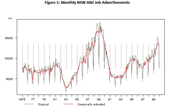
(Source for these figure 5: link)

Pseudo-Additive Decomposition:

1. The multiplicative model cannot be used when the original time series contains very small or zero values.

2. This is because it is not possible to divide a number by zero.

3.  In these cases, a pseudo additive model combining the elements of both the additive and multiplicative models is used

4. This model assumes that seasonal and irregular variations are both dependent on the level of the trend but independent of each other.

An example of series that requires a pseudo-additive decomposition model is shown below. This model is used as cereal crops are only produced during certain months, with crop production being virtually zero for one quarter each year.

pseudo-additive example

(Source for these figure 6: link)

When to which model (Additive Vs Multiplicative)?

1. Examine a graph of the original series and try a range of models, selecting the one which yields the most stable seasonal component.

2. If the magnitude of the seasonal component is relatively constant regardless of changes in the trend, an additive model is suitable.

3. If it varies with changes in the trend, a multiplicative model is the most likely candidate.

4. However if the series contains values close or equal to zero, and the magnitude of seasonal component appears to be dependent upon the trend level, then pseudo-additive model is most appropriate.

Seasonal and Irregular Chart (SI):

The following graph is an SI chart for a monthly series, using a multiplicative decomposition model:

The points represent the SIs obtained from the time series, while the solid line shows the seasonal component.

In the graph above, the SIs can be seen to fluctuate erratically, which indicates the time series under analysis is dominated by its irregular component.

A seasonal and irregular or SI chart graphically presents the SI’s for particular months or quarters in the series span. Once the trend component is estimated, it can be removed from the original data, leaving behind the combined seasonal and irregular components or SIs. The seasonal component is calculated by smoothing the SI’s, to remove irregular influences. SI charts are useful in determining whether short-term movements are caused by seasonal or irregular influences.

Before ending this article I want to share some some good articles on time series that I found:

1. Time Series Analysis with Pandas

2. Time Series Analysis: The Basics

That’s it for this article. If you have any questions feel free to ask below in the comment section. Also if you like the information provided in the article please like and subscribe to my blog. 🙂