Automatic image tilt detection using Canny edge and Hough lines and correction

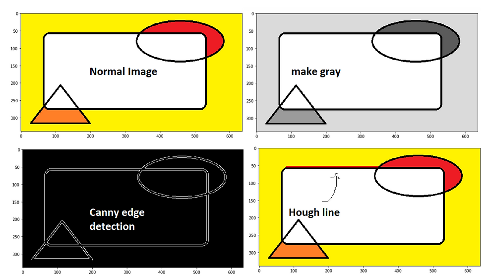
In this article we will take a look at finding during tilt angle detection of an image using Canny edges detection and Hough lines detection. I am using OpenCV functions for this purpose.

1. Explanation of Canny edges detection and Hough lines detection

2. Calculation of angle of tilt in an image

3. Correction in angle of tilted image

Where we can use this angle detection technique?

1. Applications where tilt in an image can reduce the accuracy of the algorithm and therefore we want image without tilt.

2. For example in case of Tesseract OCR with increase in tilt angle of an image the output accuracy decreases. Therefore removing tilt is necessary in such cases

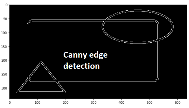
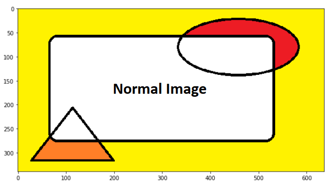
Canny edge detection

OpenCV Function is:

cv2.Canny (input_image, minVal, maxVal, aperture_size(the size of Sobel kernel used for find image gradients, By default it is 3), L2gradient: equation for finding gradient magnitude)

aperture_size:

1. It is the size of Sobel kernel used for find image gradients. By default it is 3.

2. Aperture size should be odd between 3 and 7 in function ‘Canny’

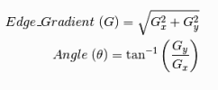
Last argument is L2gradient

1. which specifies the equation for finding gradient magnitude. If it is True, it uses the equation mentioned above which is more accurate, otherwise it uses this function: Edge_Gradient \; (G) = |G_x| + |G_y|. By default, it is False.

Example: cv2.Canny(img_gray, 100, 100, apertureSize=3)

In cv2.Canny() following steps are implemented:

Finding intensity gradients

1. Noise Reduction:

2. Since edge detection is susceptible to noise in the image, first step is to remove the noise in the image with a 5×5 Gaussian filter.

3. Finding Intensity Gradient of the Image

4. Smoothened image is then filtered with a Sobel kernel in both horizontal and vertical direction to get first derivative in horizontal direction (Gx) and vertical direction (Gy).

5. Non-maximum Suppression:

6. the result you get is a binary image with “thin edges”.

7. Hysteresis Thresholding

8. This stage decides which are all edges are really edges and which are not. For this, we need two threshold values, minVal and maxVal.

9. Any edges with intensity gradient more than maxVal are sure to be edges and those below minVal are sure to be non-edges, so discarded.

10. Those who lie between these two thresholds are classified edges or non-edges based on their connectivity. If they are connected to “sure-edge” pixels, they are considered to be part of edges. Otherwise, they are also discarded.

See the image below:

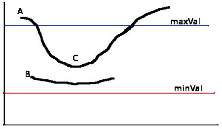
The edge A is above the maxVal, so considered as “sure-edge”. Although edge C is below maxVal, it is connected to edge A, so that also considered as valid edge and we get that full curve. But edge B, although it is above minVal and is in same region as that of edge C, it is not connected to any “sure-edge”, so that is discarded. So it is very important that we have to select minVal and maxValaccordingly to get the correct result.

This stage also removes small pixels noises on the assumption that edges are long lines. So what we finally get is strong edges in the image.

(Source)

Hough Lines

1. Hough Transform is a popular technique to detect any shape, if you can represent that shape in mathematical form.

2. It can detect the shape even if it is broken or distorted a little bit.

A line can be represented as

or in parametric form, as

where

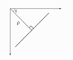
image: angle formed by this perpendicular line

1. rho is the perpendicular distance from origin to the line,

2. and  theta is the angle formed by this perpendicular line and horizontal axis measured in counter-clockwise ( That direction varies on how you represent the coordinate system. This representation is used in OpenCV). Check image

3. So if line is passing below the origin, it will have a positive rho and angle less than 180. If it is going above the origin, instead of taking angle greater than 180, angle is taken less than 180, and rho is taken negative.

4. Any vertical line will have 0 degree and horizontal lines will have 90 degree.

(rho, theta)

Now let’s see how Hough Transform works for lines:

1. Any line can be represented in these two terms, (rho, theta) .

2. So first it creates a 2D array or accumulator (to hold values of two parameters) and it is set to 0 initially.

3. Let rows denote the  rho and columns denote the theta .

4. Size of array depends on the accuracy you need.

5. Suppose you want the accuracy of angles to be 1 degree, you need 180 columns. For , the maximum distance possible is the diagonal length of the image. So taking one pixel accuracy, number of rows can be diagonal length of the image.

cv2.HoughLines (binary_image, rho, theta, threshold (minimum vote (number of points) or minimum len to consider as a line))

returns ( rho (p) and theta (angle in radians))

Parameters:

1. First parameter, Input image should be a binary image, so apply threshold or use canny edge detection before finding applying hough transform.

2. Second and third parameters are \rho and \theta accuracies respectively.

3. Fourth argument is the threshold, which means minimum vote it should get for it to be considered as a line. Remember, number of votes depend upon number of points on the line. So it represents the minimum length of line that should be detected.

1

2

3

4

5

6

7

8

9

10

11

12

13

14

15

16

17

18

19

20

21

22

23

24

25

26

27

28

29

30

31

32

33

34

35

36

37

lines = cv2.HoughLines(img_edges, 1, math.pi / 180.0, 100)

lines  #output returns ( rho (p) and theta (angle in radians))

[[[272. 1.5707964]]

[[277. 1.5707964]]

[[ 59. 1.5707964]]

[[ 54. 1.5707964]]

[[ 63. 0. ]]

[[ 68. 0. ]]

[[529. 0. ]]

[[534. 0. ]]

[[318. 1.5707964]]

[[313. 1.5707964]]

[[214. 0.6632251]]

[[ 51. 1.5882496]]

[[ 35. 2.4783676]]

[[219. 0.6632251]]

[[ 61. 1.553343 ]]

[[279. 1.553343 ]]

[[270. 1.5882496]]

[[ 40. 2.4783676]]]

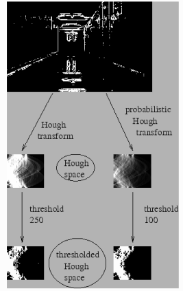
Hough LinesP

1. Probabilistic Hough Transform

2. In the hough transform, you can see that even for a line with two arguments, it takes a lot of computation.

3. Probabilistic Hough Transform is an optimization of Hough Transform we saw.

4. It doesn’t take all the points into consideration, instead take only a random subset of points and that is sufficient for line detection.

5. Just we have to decrease the threshold.

Source

cv2.HoughLinesP(binary_image, rho, theta, threshold, minLineLength, maxLineGap)

Where:

1. threshold (minimum vote (number of points) or minimum len to consider as a line)

2. minLineLength: Line segments shorter than this are rejected

3. maxLineGap: Maximum allowed gap between line segments to treat them as single line

Example:

1

2

3

4

5

6

7

8

9

10

11

12

13

14

15

16

17

18

19

20

21

22

23

linesP = cv2.HoughLinesP(img_edges, 1, math.pi / 180.0, 100, minLineLength=100, maxLineGap=5)

linesP

[[[ 79 54 343 54]]

[[173 277 520 277]]

[[ 80 59 337 59]]

[[168 272 520 272]]

[[ 63 268 63 70]]

[[534 264 534 130]]

[[ 68 259 68 71]]

[[ 26 318 201 318]]

[[529 263 529 69]]

[[ 27 313 191 313]]

[[ 34 312 117 206]]]

Calculating angle

1. Once we have hough lines. For any one line we can calculate angle of that line since we know the end points (x1, y1) and (x2, y2) of that line.

2. Hence we can find angle of line connecting (0,0) to (x,y) from +ve x axis

Example:

1

2

for x1, y1, x2, y2 in lines[0]: #calculating tilt angle

angle = math.degrees(math.atan2(y2 - y1, x2 - x1))  # find angle of line connecting (0,0) to (x,y) from +ve x axis

Now we have enough information about these steps. For end-to-end image tilt angle detection please refer this code on my GitHub repository.

If you have any question feel free to ask in the comment section below. Also please like and subscribe to my blog. 🙂